This work is preregistered and has a study protocol [3] which is considered a useful manner of working but currently rare in epidemic modelling. The protocol outlines the modelling considerations we made before work began and may serve as a useful resource for the interested reader.
Data
In this work we consider daily data (\(t = 1, \ldots , 312 = T\)) where the study period commences on 24th February 2020 and the final observation at time T occurs on 31st December 2020. COVID-19 case data is provided by the Swiss public health authority (Bundesamt für Gesundheit) and includes case counts by date reported stratified by age group. We asked for cases given by the same age groups we considered in our Zurich analysis as this roughly divides the population into those of compulsory education age including compulsory kindergarten/pre-school/reception (0–14 year olds), higher education and young workers (15–24), parents (25–44), middle-aged workers (45–65), retirees (66–79), and the elderly (80+). Our age group thresholds include the commonly used cut-off of 65 years of age considered in epidemiology, when health is expected to change.
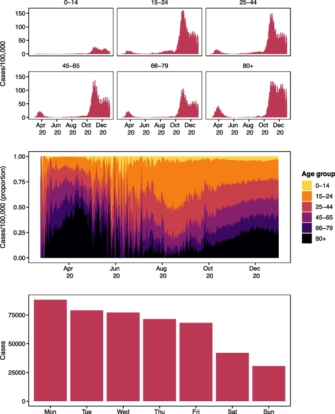
Figure 1 shows the case data; the daily number of cases per 100,000 age group population (upper panel), the distribution of cases per 100,000 population over time (middle panel), and cases by weekday reported (lower panel). The upper panel shows the oscillatory behaviour known to epidemic curves as well as weekly systematic fluctuations in surveillance. The middle panel shows a shift in the age distribution of cases across the study period which further motivates the inclusion of age groups in our modelling approach. The lower panel shows the distribution of cases across the days of the week, where we see a systematic fluctuation in the reporting system. The legal workdays in Switzerland are Monday through Friday. Most cases are reported on Mondays which is the start of the week according to European norms and the number of reported cases drops across the week while fewer cases are reported on weekends (Saturday and Sunday).
To capture baseline transmission opportunities between age groups we include a contact matrix in our endemic-epidemic model. Contact matrices encapsulate the number of contacts an average person in the population has with other population members of the same and different ages in different settings such as the workplace or school. Their inclusion in the endemic-epidemic framework was an approach introduced by Meyer and Held [17] which provided more realism than making an assumption of mixing patterns for the population. Existing contact diary-based contact matrices for Switzerland are only based on a small number of observations (54 observations) [15], which led us to use a synthetic contact matrix in place of this empirical one. A synthetic contact matrix is constructed on the basis of demographic information. In particular national statistics on household composition, average school class size, age, and employment is used to create a synthetic population. The contact network of this synthetic population is used to determine the contact matrix. Finally, the synthetic contact matrix is calibrated with empirical matrices created for Europe. An overview of other developments for contact matrices can be found in Bekker-Nielsen Dunbar [1].
We chose to use the synthetic matrices by Mistry et al. [18] as they were both 1) newer and 2) given with a certain level of uncertainty which we could incorporate into our modelling approach. The synthetic contact matrix is constructed on the basis of household size, school enrolment records, and employment data (see [18], for details).
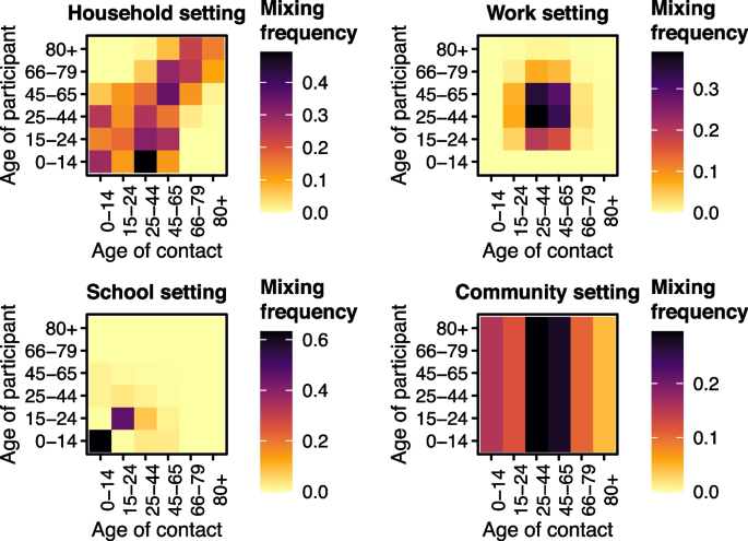
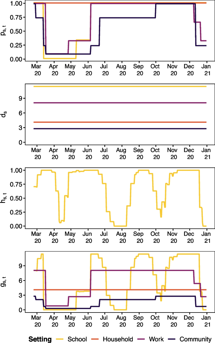
From the synthetic contact matrix we obtain the per capita relative frequency of contact \(c_{a, a’, s}\) between age group a and age group \(a’\) in setting s (shown in Fig. 2 which describes the pattern of mixing in each setting considered) and the disease-specific weights \(d_s\) in setting s for constructing contact matrices for respiratory disease, which are 4.11 for household setting, 11.41 for school setting, 8.07 for work setting, and 2.79 for general community setting (shown in Fig. 3). This means school has the largest weight and so changes to these contacts are expected to have the biggest impact. In high income countries (of which Switzerland has the highest income globally), most contacts occur in educational settings [19], so the choice does not seem unreasonable. These construction weights \(d_s\) are provided with standard errors. When constructing \(c_{a, a’}\) we used the Swiss population (Table 1) rather than the Zurich population which we considered in earlier work (see [2], for the analysis of Zurich) such that the population used to weight the synthetic contact matrix was the one being studied. This means the contact matrix used in this work is not exactly the same as the one considered previously. The Mistry et al. [18] contact matrices are created with respiratory diseases in mind where school closure is a first line of defence against disease outbreaks. The synthetic contact matrix was used to inform the time-varying transmission weights \(w_{a, a’, t}\) which determine the amount of transmission between age group a and age group \(a’\) at time t, which is explained in more detail below.
Contact setting-specific daily policy adjustments \(p_{s,t}\) are informed by information provided by the Swiss authorities. This information is used to quantify the amount of disease control measures enacted. We focus on those measures which have the aim to decrease contact. Following the Oxford University policy classifications we consider: school closure (“C1”), workplace closure (“C2”), and restrictions on gatherings (“C4”). We code our policy indicators to take the same levels as the Oxford scheme allowing researchers familiar with the controlled vocabulary established by that research group to comprehend our indicators. We reversed and rescaled the indicators such that \(p_{s, t}\in [0, 1]\) where 0 reflects a situation of maximal measures in place and 1 is full relaxation of measures (source information is in our study protocol https://osf.io/fgrdy).
The non-pandemic school closure adjustment \(h_{s,t}\) is created based on information from Schweizerische Konferenz der kantonalen Erziehungsdirektoren [23] and reflects closures of school during the academic year due to half term and other school holidays. These closures reduce contact independently of disease control measures; notably Easter is a period where less contacts in school settings would be expected as Switzerland is a predominantly Christian country. The adjustment takes values \(h_{s,t}\in [0,1]\) where 0 means that all schools in Switzerland are closed on that day and 1 means all schools are open. The values \(h_{s,t}\) takes for the school setting are shown in Fig. 3 while \(h_{s,t}\equiv 1\) for all other contact settings (meaning no adjustment). The calculation of \(h_{s,t}\) is informed by population data from Eurostat [11] (population by region). The construction of \(p_{s,t}\), \(h_{s,t}\), and \(w_{a,a’,t}\) is explained in more detail in the following section.
Model
The endemic-epidemic model is a time series regression model used for infectious disease surveillance which sees frequent use for applications which require the incorporation of transmisson between population strata [12, 20, 26]. In an age-stratified endemic-epidemic model, case counts \(Y_{at}\) are indexed by time t and age group a. The age groups considered are 0–14, 15–24, 25–44, 45–65, 66–79, and 80+ years; the same used in Bekker-Nielsen Dunbar et al. [2]. Case counts given past cases are assumed to follow an overdispersed negative binomial distribution with age-dependent overdispersion parameters \(\psi _a\). The mean \(\lambda _{at}\) is additively decomposed into endemic and epidemic components. Log-linear predictors for the endemic and epidemic components are given by \(\nu _{at}\) and \(\phi _{at}\) respectively. The endemic component is additionally weighted by population fractions \(e_a\), where we used population data from Eurostat [10] (population by age group), given in Table 1 to inform this part of the model. This functions as a model offset (see [17], for description of model offsets).
The epidemic component is an autoregressive process additionally driven by cases in other age groups \(a’\) in previous time periods \(t – \ell\) up to a maximum lag of \(\ell _{\text {max}}\) where \(u_\ell\) determines by how much previous cases are weighted. We chose to use a Poisson-distributed lag distribution \(u_\ell\) such that the majority of the weight need not be given to the immediately preceeding cases allowing for a serial interval of more than a single day. The maximum lag represents the maximum length of the serial interval we might conceive in our modelling efforts; we chose \(\ell _{\text {max}} = 7\) as the literature suggests early types of COVID-19 have a serial interval within a week [21].
Our endemic-epidemic model with time dependent [2, 13] contact matrix weights [17] and higher order lag [5] is given by
$$\begin{aligned} Y_{at} \mid Y_{a, t – 1}, \ldots , Y_{a, t – \ell _{\text {max}}} & \sim \text {NegBin}(\lambda _{at}, \psi _a) \nonumber \\ \lambda _{at} & = \underbrace{\nu _{at} e_{a}}_{\text {endemic}} + \underbrace{\phi _{at} \sum \limits _{a’}\sum \limits _{\ell = 1}^{\ell_{\text {max}}} u_\ell w_{a, a’, t} Y_{a’, t – \ell }}_{\text {epidemic}} \nonumber \\ u_\ell & \propto \frac{\kappa ^ {\ell – 1}}{(\ell – 1)!} \cdot \exp (- \kappa ), \quad \kappa > 0, \ell = 1, \ldots , \ell _{\text {max}} \end{aligned}$$
(1)
Transmission between age groups is determined by a time-dependent contact matrix \(w_{a, a’, t}\). The time-varying contact matrix \(w_{a, a’, t}\) is the total average contacts at time t constructed by a weighted sum
$$\begin{aligned} w_{a, a’, t} = \sum \limits _s g_{s, t} \cdot c_{a, a’, s} \end{aligned}$$
(2)
where \(g_{s, t}\) is a weight that depends on the setting s the contact occurred in and changes occuring at time t. It is created from the combination of the weights used to construct contact matrices (\(d_s\) given by Mistry et al. [18] which depend on setting s), the time-dependent setting-specific policy adjustments (\(p_{s,t}\) which depend on time t and setting s) and whether an adjustment needs to be made to incorporate non-pandemic school closure due to school holidays (\(h_{s,t}\) which depends on setting s as it only affects schools and time t):
$$\begin{aligned} g_{s, t} = d_s \cdot p_{s, t} \cdot h_{s, t} \end{aligned}$$
(3)
Since school holidays in Switzerland vary not only between regions, but also within them, we construct binary indicators for all of the sub-regions r within a region R where we assign 1 to a specific day t if t is not a school holiday and 0 otherwise. In a second step, we average the binary indicators of all sub-regions r within a region R in order to obtain a regional average indicator for that day. Subsequently, we use population weights to calculate the national indicator \(h_{s, t}\). The sub-regions are unweighted in our averaging as we were not able to determine population sizes at school district level. We calculate
$$\begin{aligned} h_{s, t} = \left\{\begin{array}{ll}\sum \nolimits _{R}\frac{\sum \nolimits _{r\in R} \mathbbm{1}_{\{t\ \text {is}\ not\ \text {a school holiday in subregion}\ r\}}(t) \, / n_R}{\text {population}_{R}} & s = \text {school} \\ 1 & \text {otherwise} \end{array} \right.\ \end{aligned}$$
(4)
where \(\mathbbm{1}\) is an indicator function and \(n_R\) denotes the number of sub-regions within region R. This gives us a population-weighted indicator with values \(h_{s,t}\in [0, 1]\) which incorporates the variation of number of school children in regions.
We fit the model (1) with predictors
$$\begin{aligned} \log (\nu _{at}) & = \alpha ^{(\nu )}_a + \beta ^{(\nu )}_1 x_{1t} + \beta _2^{(\nu )} x_{2t} + \gamma ^{(\nu )} \sin (2\pi t/365 + \delta ^{(\nu )}) \nonumber \\ \log (\phi _{at}) & = \alpha ^{(\phi )}_a + \beta ^{(\phi )}_1 x_{1t} + \mathbf {\beta _2^{(\phi)\mathrm{T}}} \textbf{z}_t + \gamma ^{(\phi )} \sin (2\pi t/365 + \delta ^{(\phi )}) \end{aligned}$$
(5)
where \(\alpha _a\) denotes a fixed effect of age group a, \(x_{1t}\) is an indicator for public holidays, \(x_{2t}\) is an indicator for weekends, and \(\textbf{z}_t\) are effect-coded weekday effects with Monday as the reference value (six in total). Effect-coded variables are also known as sum-to-zero contrasts. This means Monday always takes the value \(-1\) and the weekday of interest takes the value 1 while all other weekdays are 0. We include a non-linear time trend in the form of a sinusoidal wave expressed by its amplitude \(\gamma\) and phase \(\delta\) [22]. Our model has 31 parameters (estimates are given in Table 3) which are estimated using a maximum likelihood approach computed with standard errors. Information on the full model selection procedure (where we also considered effects of temperature, testing rate, and a linear time trend) can be found in the supporting information.
Counterfactual scenario prediction
Determining the expected size of the outbreak is crucial to policy makers who need to determine how resources are to be allocated. As the outbreak is ongoing, the predicted final size considered here is the predicted number of infections over the time window considered rather than the traditional metric used by compartmental modellers: the total number of infections over the entire outbreak period. Predicted cases are based on a path trajectory (a long-term expected prediction calculated recursively on the basis of one-step predictions) following Held et al. [14] assuming no changes to the model parameters across the scenarios considered. This means we predict the model (1) with the given \(e_{a}\) and fitted \(\hat{\nu }_{at}\), \(\hat{\phi }_{at}\), and \(\hat{u}_\ell\) effects for three different versions of \(w_{a, a’, t}\) (for scenarios A, B, and C). The two counterfactual scenarios are implemented by including transmission weights informed by \(g_{s, t, a, a’} = d_s \cdot q_{s, t, a, a’} \cdot h_{s, t}\) where g now depends on age group. In particular we consider three scenarios (provided with the shorthand names we use based on their effect on the youngest age group):
-
Scenario A (“true measures”) This is the true measures scenario where schools closed in the spring and reopened in the summer where \(w_{a, a’, t}\) is populated by the relevant policy information without adjustment as in (2). This is the same scenario considered in model fitting to obtain the model coefficients used in prediction of final size and simulation of uncertainty for the prediction.
-
Scenario B (“schools open”) This is a scenario where schools are never closed for the youngest age group (0–14), i.e. remain open across the entire study period. All other measures are as in Scenario A.
$$\begin{aligned} q_{s, t, a, a’} = \left\{ \begin{array}{ll} 1 & a = \text {0-14} \, \text {or} \, a’ = \text {0-14} \, \text {and} \, s = \text {school}\\ p_{s, t} & a \ne \text {0-14} \, \text {and} \, a’ \ne \text {0-14} \, \text {and} \, s = \text {school}\\ p_{s, t} & s\ne \text {school} \end{array}\right. \end{aligned}$$
(6)
-
Scenario C (“schools closed”) This is a scenario where schools close and remain closed. School closure once again affects age group 0–14 and their contacts. All other measures are as in Scenario A. We implement this by setting
$$\begin{aligned} q_{s, t, a, a’} = \left\{ \begin{array}{ll} p_{s, t} & t < t_0 \text { and } a = \text {0-14} \, \text {or} \, a’ = \text {0-14} \text{ and } s = \text {school} \\ p_{s, t} & a \ne \text {0-14} \, \text {and} \, a’ \ne \text {0-14} \text{ and } s = \text {school} \\ 0 & t \ge t_0 \text { and } a = \text {0-14} \, \text {or} \, a’ = \text {0-14}\ \text {and}\ s = \text {school} \end{array}\right. \end{aligned}$$
(7)
where \(t_0\) denotes the date schools are first closed (16th March 2020).
The changes only affect age group 0–14 when the contact matrix is multiplied by \(g_{s, t, a, a’}\) so the 0–14 row and column in Fig. 2 are changed in the school setting (school aged children and their contacts). The time series of all four setting-specific policy indicators \(p_{s, t}\) can be seen in Fig. 3 (the building blocks of (2), (6), (7)). The truth (scenario A) is expected to lie somewhere between the two counterfactual scenarios (scenarios B and C), see Table 2. Examining the deviation these scenarios have allows us to evaluate the effect of disease control measures used. It is implicitly assumed that the fitted effects \(\hat{\nu }_{at}\), \(\hat{\phi }_{at}\), \(\hat{u}_{\ell}\) do not vary across scenarios.
To incorporate parameter uncertainty in our projections, we utilise Monte Carlo simulation. We sample the weights \(d_s\) with uncertainty estimates given in Mistry et al. [18] assuming they are independently normally distributed. To incorporate model uncertainty we sample the coefficients \(\hat{\nu }_{at}\), \(\hat{\phi }_{at}\), \(\hat{\psi }_{a}\), \(\hat{\kappa }\), of our fitted endemic-epidemic model assuming a multivariate normal distribution; the asymptomatic normal distribution of the maximum-likelihood estimates. Using these \(n = 1000\) samples we then use the path trajectory prediction approach to obtain n simulated expected case counts under the scenarios considered. This enables us to incorporate uncertainty in our projections. We examine the expected increase in cases when schools are always open (scenario B) and the expected decrease in cases when schools are always closed (scenario C) and compare this with the expected number of cases under the policy used (scenario A).
We also conducted sensitivity analyses of the assumptions made in constructing the transmission weights \(w_{a,a’,t}\). The sensitivity analyses attempt to provide further realism with respect to how household contacts may be affected by school closure. This provides additional extensions to the analysis of Zurich data as here we only considered household contacts to not be affected by policy \(p_{s, t}\vert _{s=\text {household}}\equiv 1\). The sensitivity analyses can be found in the supporting information.


